Duration
About 3 hours
You set every stage timing from the professor panel, so it fits one block or splits across two sessions.
Behavioral Biases in Investment Decisions Simulation
The Finsimco Behavioral Biases Simulation asks each student forty questions that are arithmetically identical in pairs, then shows them their own answers and fits the curve those answers produced.
Duration
You set every stage timing from the professor panel, so it fits one block or splits across two sessions.
Format
Each student holds the choice, measurement and design roles in turn and submits one committee process.
Level
Adjustable: twenty bets with simple framing, up to forty bets, a moved reference point and an ambiguity test.
Professor tools
Manage students, adjust stage timings, control progression and monitor individual inputs.
Prerequisites
Students need to be comfortable with probabilities. Prospect theory and framing are taught inside.
Delivery
The web-based simulation supports in-person, remote, blended and homework-supported delivery.
Assessment
Every submission is individual, so the forty answers, the committee design and the review answers export per student.
Course fit
Designed for Behavioural Finance, Investments, Decision Science and Managerial Economics courses.
The topics a behavioral biases in investment decisions module has to cover: prospect theory and the value function, loss aversion and its coefficient, framing effects, reference points and how they move, probability weighting and designing a process that constrains a bias.
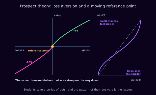
The prospect theory value function. Gains and losses are measured from a reference point rather than from any absolute level of wealth, and the value placed on them runs up the side. The curve is concave in gains, so the second thousand feels like less than the first, and convex in losses, which is why people double down. The loss side is about twice as steep, so losing a thousand dollars feels roughly twice as bad as gaining one feels good. Beside it is the probability weighting curve: small chances overweighted, large ones underweighted.
Written to drop into your module descriptor without rewriting. On completing the simulation, your students will be able to:
Each student answers alone, holding the choice, measurement and design roles in turn. All three want something different from the same forty answers, and only one process design is submitted.
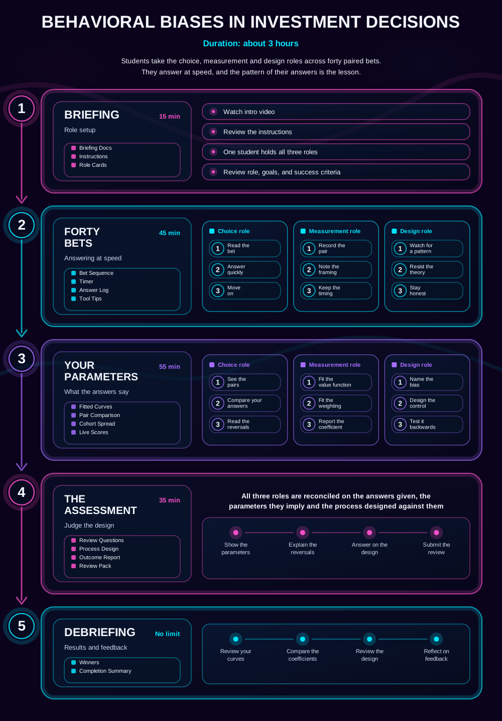
The gameflow every student sees before they start. The three roles come into play across the bets and the fitting; briefing, the assessment and the debrief are worked as a single view. Materials arrive stage by stage: instructions and role cards at briefing, then the bet sequence and answer log, then the fitted curves, pair comparison and cohort spread.
Students work through forty paired bets at speed, because the effect disappears if there is enough time to notice the pairs are the same.
Students fit a value function and a weighting function to their own answers, which turns a lecture topic into a personal coefficient.
Students build a committee procedure that would have produced a different answer from the one they just gave.
Five stages. Students answer forty bets, have their own parameters fitted and design a process against them.
Briefing Docs · Instructions · Role Cards
Briefing
Students watch the intro video, review a short set of instructions that deliberately does not say what is being measured, and take on all three roles, checking the timing and the success criteria before the first question appears.
Bet Sequence · Timer · Answer Log · Tool Tips
Forty Bets
Forty bets run under a timer. Twenty pairs are arithmetically identical and differently framed, some from a gain position and some from a loss, some with small probabilities and some with large, and the timing is deliberately tight enough that the pairs are not spotted.
Fitted Curves · Pair Comparison · Cohort Spread · Live Scores
Your Parameters
The answers are fitted. The student's own loss aversion coefficient and probability weighting curve are estimated, the reversals between identical pairs are listed, and the student then designs a committee process intended to produce the answer their own data says they would not have given.
Review Questions · Process Design · Outcome Report · Review Pack
The Assessment
The design is assessed. Students are asked what their loss aversion coefficient was, which pair they reversed most sharply, whether their committee process would have changed any of their own answers, and what it would cost in time to run.
Winners · Completion Summary
Debriefing
Students review their own fitted curves, compare coefficients across the cohort, revisit the reversals that separated them and reflect on the feedback. Winners and the completion summary give you a structure for the discussion.
The student interface carries the bets, the fitted curves and the design. The professor panel carries the timeline, the controls and every individual coefficient.
Students answer under a timer, with the two options and their probabilities side by side, and the paired question deliberately placed several items away.
The reversal list is the one that lands. Eleven of twenty pairs were answered differently, and the pairs were arithmetically identical.
Your view. Adjust any stage timing, start or stop the session, and compare the coefficients across the cohort before the theory is introduced.
Explore the student and professor experience, and discuss timing, setup and syllabus fit.
It works best as the session that produces the data the lecture then explains.
Comfort with probabilities. Prospect theory, loss aversion and probability weighting are explained after the answers are collected.
Early module, typically weeks one to four, before prospect theory is formally taught.
Market anomalies, investor behaviour, nudges and choice architecture, adviser conduct, and any assessment asking students to apply behavioural theory.
The behavioural biases course guide sets out where it sits in a full module.
The three mistakes students make on this case, and what each one gives you in the debrief. Our simulations are designed around them: read the learning science behind it.
1
A student who recognises the pair answers consistently and learns nothing. The timing exists to prevent this, and the cohorts that take the bets slowly produce flat curves and a disappointing session.
2
A loss-averse person takes more risk when behind and less when ahead, which is the opposite of what a risk-averse person does. Students use the two words interchangeably until their own answers separate them.
3
Telling a committee about loss aversion changes nothing, as the literature is very clear about. A control is a procedure that produces a different answer, such as requiring every position to be re-argued from a zero reference point.
The debrief runs itself. Every student sees their results, the cohort comparison and the decisions that produced them, with nothing for you to prepare. If you would rather lead the discussion, these questions work straight from a slide, and they use what your cohort actually did.
Assessment is optional. Run the simulation ungraded as an applied activity, or use platform data as supporting evidence. Every student generates forty answers, fitted parameters, a committee process design and written rationales. Because the simulation is single-player, every input belongs to one named student, so there is no group-work marking to untangle. All of it exports as CSV or PDF, per student, so you can assess reasoning rather than a result.
On generative AI: written rationales are exactly what marking teams now worry about. Because every answer here is recorded inside the platform under a timer and before any theory is introduced, the data behind the reasoning is the student's own.
93% of students rate Finsimco simulations Excellent, across more than 30,000 responses.
Teaching notes, a setup and facilitation guide and a gameflow diagram come with it, and we support your first delivery directly.
Run it ungraded the first time. Assessment is optional and can be added once you have seen how your cohort responds.
Pause or stop at any point and resume later without losing submitted data, so an overrun costs you a timetable slot, not the activity.
Read what lecturers say.
Ron Tuninga, Managing Director for EMEA at AACSB, and Victor Hedenberg, Membership Director at AMBA, on why simulation-based learning belongs in business education. Watch both interviews.
If this one is not quite right for your module, these are the closest alternatives.
A one-page summary of this simulation, covering stages and timings, roles, concepts, learning outcomes and the debrief questions, plus a full sample teaching pack from one of our live simulations, so you can see exactly what you would be running.
During the call, we can:


